Intro to Tensorflow and Keras for CSS Scholars
Last modified: 2022/04/24
Description: Everything you need to know to use Keras & TensorFlow for deep learning research.
Disclosure: This tutorial is based on https://keras.io/getting_started/intro_to_keras_for_researchers/
What is TensorFlow?
 </br>
</br>
TensorFlow is a free and open-source software library for dataflow and differentiable programming. It is a symbolic math library used for machine learning applications such as neural networks.
TensorFlow was developed by the Google Brain team for internal Google use. Open Sourced November 2015.
TensorFlow handles tensor, tf variables, and gradients.
What is Keras?
![]() </br>
</br>
Keras is an open-source library that provides a Python interface for artificial neural networks. Keras acts as an interface for the TensorFlow library. So Keras is a high level API that deals with models, layers, optimization, etc. It contains numerous implementations of commonly used neural-network building blocks such as layers, objectives, activation functions, optimizers, and a host of tools for processsing image and text data.
If you go to this page, you can see all Keras API references https://keras.io/api/:
Models API (Sequential class, Model training APIs, Model saving & serialization APIs)
Layers API (base layers, core layers, covlayers, pooling layers, activation, locally connected layers etc.)
Callbacks API (base Callback class, ModelCheckpoint, TensorBoard, EarlyStopping, etc)
Data preprocessing (Image data preprocessing, Text data preprocessing)
Optimizers (SGD, RMSprop, Adam, Adadelta, Adagrad, Adamax, etc)
Metrics (Accuracy metrics, Probabilistic metrics, Regression metrics, Classification metrics based on True/False)
Losses (Probabilistic losses, Regression losses, Hinge losses for "maximum-margin" classification)
Built-in small datasets (MNIST digits classification dataset, CIFAR10 small images classification dataset, CIFAR100, small images classification dataset, IMDB movie review sentiment classification dataset, Reuters newswire classification dataset, Fashion MNIST dataset, an alternative to MNIST, Boston Housing price regression dataset)
Keras Applications (Xceptionm EfficientNet B0 to B7, VGG16 and VGG19, ResNet and ResNetV2, MobileNet and MobileNetV2, DenseNet, NasNetLarge and NasNetMobile, InceptionV3, InceptionResNetV2)
Note: check CIFAR https://www.cs.toronto.edu/~kriz/cifar.html
Let us get it started!!!
Installation
pip install "tensorflow>=2.0.0"
Will get you setup for CPU-only, vanilla TensorFlow, including the Tensorflow version of Keras
TensorFlow has very wide spectrum of possible optimization
GPU, Cluster, optimized execution ordering, vector processing instructions, ....
Compile yourself to get higher efficiency
Also make sure you have the PyLab stack
pip install scipy numpy matplotlib
Additional recommended Python tools to make this comfortable are iPython and Jupyter Lab
pip install ipython jupyter
import tensorflow as tf
from tensorflow import keras
import numpy as np
Introduction
In this guide, you will learn about:
- Tensors, variables, and gradients in TensorFlow
- The Keras Sequential API
- The Keras Functional API
You will also see the Keras API in action in two end-to-end research examples: Train a simple neural network and use pretrained models to do transfer learning.
Tensors
TensorFlow is an infrastructure layer for differentiable programming. At its heart, it's a framework for manipulating N-dimensional arrays (tensors), much like NumPy.
However, there are three key differences between NumPy and TensorFlow:
- TensorFlow can leverage hardware accelerators such as GPUs and TPUs.
- TensorFlow can automatically compute the gradient of arbitrary differentiable tensor expressions.
- TensorFlow computation can be distributed to large numbers of devices on a single machine, and large number of machines (potentially with multiple devices each).
Let's take a look at the object that is at the core of TensorFlow: the Tensor.
Here's a constant tensor:
x = tf.constant([[5, 2], [1, 3]])
print(x)
You can get its value as a NumPy array by calling .numpy():
x.numpy()
Much like a NumPy array, it features the attributes dtype and shape:
print("dtype:", x.dtype)
print("shape:", x.shape)
print(2**32)
A common way to create constant tensors is via tf.ones and tf.zeros (just like np.ones and np.zeros):
print(tf.ones(shape=(2, 1)))
print(tf.zeros(shape=(2, 1)))
You can also create random constant tensors:
x = tf.random.normal(shape=(2, 2), mean=0.0, stddev=1.0)

x = tf.random.uniform(shape=(2, 2), minval=0, maxval=10, dtype="int32")
Variables
Variables are special tensors used to store mutable state (such as the weights of a neural network).
You create a Variable using some initial value:
initial_value = tf.random.normal(shape=(2, 2))
a = tf.Variable(initial_value)
print(a)
You update the value of a Variable by using the methods .assign(value), .assign_add(increment), or .assign_sub(decrement):
new_value = tf.random.normal(shape=(2, 2))
a.assign(new_value)
for i in range(2):
    for j in range(2):
        assert a[i, j] == new_value[i, j]

added_value = tf.random.normal(shape=(2, 2))
a.assign_add(added_value)
for i in range(2):
    for j in range(2):
        assert a[i, j] == new_value[i, j] + added_value[i, j]
Doing math in TensorFlow
If you've used NumPy, doing math in TensorFlow will look very familiar. The main difference is that your TensorFlow code can run on GPU and TPU.
a = tf.random.normal(shape=(2, 2))
b = tf.random.normal(shape=(2, 2))

c = a + b
d = tf.square(c)
e = tf.exp(d)
print(e)
Gradients
Here's another big difference with NumPy: you can automatically retrieve the gradient of any differentiable expression.
Just open a GradientTape, start "watching" a tensor via tape.watch(),
and compose a differentiable expression using this tensor as input:
a = tf.random.normal(shape=(2, 2))
b = tf.random.normal(shape=(2, 2))

with tf.GradientTape() as tape:
    tape.watch(a)  # Start recording the history of operations applied to `a`
    c = tf.sqrt(tf.square(a) + tf.square(b))  # Do some math using `a`

# What's the gradient of `c` with respect to `a`?
dc_da = tape.gradient(c, a)
print(dc_da)
By default, variables are watched automatically, so you don't need to manually watch them:
a = tf.Variable(a)

with tf.GradientTape() as tape:
    c = tf.sqrt(tf.square(a) + tf.square(b))
    dc_da = tape.gradient(c, a)
    print(dc_da)
Note that you can compute higher-order derivatives by nesting tapes:
with tf.GradientTape() as outer_tape:
    with tf.GradientTape() as tape:
        c = tf.sqrt(tf.square(a) + tf.square(b))
        dc_da = tape.gradient(c, a)
    d2c_da2 = outer_tape.gradient(dc_da, a)
    print(d2c_da2)
Keras layers
While TensorFlow is an infrastructure layer for differentiable programming, dealing with tensors, variables, and gradients, Keras is a user interface for deep learning, dealing with layers, models, optimizers, loss functions, metrics, and more.
Keras serves as the high-level API for TensorFlow: Keras is what makes TensorFlow simple and productive.
The Layer class is the fundamental abstraction in Keras.
A Layer encapsulates a state (weights) and some computation
(defined in the call method).
Neural Networks go back and forth between two stages:
- Linear model $x \to Wx + b$
- Non-linear activation function $x \to f(x)$
A simple layer looks like this:
Note that if you are not familiar with python classes, you can click here for more info https://docs.python.org/3/tutorial/classes.html
class Linear(keras.layers.Layer):
    """y = w.x + b"""

    def __init__(self, units=32, input_dim=32):
        super(Linear, self).__init__()
        # tf.random_normal_initializer(mean=0.0, stddev=0.05, seed=None)
        w_init = tf.random_normal_initializer()
        self.w = tf.Variable(
            initial_value=w_init(shape=(input_dim, units), dtype="float32"),
            trainable=True
        )
        b_init = tf.zeros_initializer()
        self.b = tf.Variable(
            initial_value=b_init(shape=(units,), dtype="float32"), trainable=True
        )

    def call(self, inputs):
        return tf.matmul(inputs, self.w) + self.b
You would use a Layer instance much like a Python function:
# Instantiate our layer.
linear_layer = Linear(units=4, input_dim=2)

# The layer can be treated as a function.
# Here we call it on some data.
y = linear_layer(tf.ones((2, 2)))
assert y.shape == (2, 4)
print(y)
You have many built-in layers available, from Dense to Conv2D to LSTM to
fancier ones like Conv3DTranspose or ConvLSTM2D.
Layer weight creation
The self.add_weight() method gives you a shortcut for creating weights:
class Linear(keras.layers.Layer):
    """y = w.x + b"""

    def __init__(self, units=32):
        super(Linear, self).__init__()
        self.units = units

    def build(self, input_shape):
        self.w = self.add_weight(
            shape=(input_shape[-1], self.units),
            initializer="random_normal",
            trainable=True,
        )
        self.b = self.add_weight(
            shape=(self.units,), initializer="random_normal", trainable=True
        )

    def call(self, inputs):
        return tf.matmul(inputs, self.w) + self.b


# Instantiate our lazy layer.
linear_layer = Linear(4)

# This will also call `build(input_shape)` and create the weights.
y = linear_layer(tf.ones((2, 2)))
print(y)
Layer gradients
You can automatically retrieve the gradients of the weights of a layer by
calling it inside a GradientTape. Using these gradients, you can update the
weights of the layer, either manually, or using an optimizer object. Of course,
you can modify the gradients before using them, if you need to.
# Prepare a dataset.
# Keras has many built-in datasets. Now we load mnist handwritten digits data
(x_train, y_train), _ = tf.keras.datasets.mnist.load_data()
# this load_data function returns
# Tuple of Numpy arrays: (x_train, y_train), (x_test, y_test).
# x_train, x_test: uint8 arrays of grayscale image data with shapes (num_samples, 28, 28).
# y_train, y_test: uint8 arrays of digit labels (integers in range 0-9) with shapes (num_samples,).

# The tf.data.Dataset API supports writing descriptive and efficient input pipelines.
# Dataset usage follows a common pattern:
# Create a source dataset from your input data.
# Apply dataset transformations to preprocess the data.
# Iterate over the dataset and process the elements.
# Iteration happens in a streaming fashion, so the full dataset does not need to fit into memory.
# check here for other details <https://www.tensorflow.org/api_docs/python/tf/data/Dataset>

dataset = tf.data.Dataset.from_tensor_slices(
    (x_train.reshape(60000, 784).astype("float32") / 255, y_train)
)

# shuffle the data (randomize the data)
# Combines consecutive elements of this dataset into batches
dataset = dataset.shuffle(buffer_size=1024).batch(64)

# Instantiate our linear layer (defined above) with 10 units.
linear_layer = Linear(10)

# Instantiate a logistic loss function that expects integer targets.
# check here for loss function <https://www.tensorflow.org/api_docs/python/tf/keras/losses/SparseCategoricalCrossentropy>
loss_fn = tf.keras.losses.SparseCategoricalCrossentropy(from_logits=True)

# Instantiate an optimizer.
# check here for the SGD optimization <https://www.tensorflow.org/api_docs/python/tf/keras/optimizers/SGD>
optimizer = tf.keras.optimizers.SGD(learning_rate=1e-3)

# Iterate over the batches of the dataset.
for step, (x, y) in enumerate(dataset):

    # Open a GradientTape.
    with tf.GradientTape() as tape:

        # Forward pass.
        logits = linear_layer(x)

        # Loss value for this batch.
        loss = loss_fn(y, logits)

    # Get gradients of weights wrt the loss.
    gradients = tape.gradient(loss, linear_layer.trainable_weights)

    # Update the weights of our linear layer.
    optimizer.apply_gradients(zip(gradients, linear_layer.trainable_weights))

    # Logging.
    if step % 100 == 0:
        print("Step:", step, "Loss:", float(loss))
Tracking losses created by layers
Layers can create losses during the forward pass via the add_loss() method.
This is especially useful for regularization losses.
The losses created by sublayers are recursively tracked by the parent layers.
Here's a layer that creates an activity regularization loss:
class ActivityRegularization(keras.layers.Layer):
    """Layer that creates an activity sparsity regularization loss."""
    # https://www.tensorflow.org/api_docs/python/tf/keras/layers/ActivityRegularization

    def __init__(self, rate=1e-2):
        super(ActivityRegularization, self).__init__()
        self.rate = rate

    def call(self, inputs):
        # We use `add_loss` to create a regularization loss
        # that depends on the inputs.
        self.add_loss(self.rate * tf.reduce_sum(inputs))
        return inputs
Any model incorporating this layer will track this regularization loss:
# Let's use the loss layer in a MLP block.


class SparseMLP(keras.layers.Layer):
    """Stack of Linear layers with a sparsity regularization loss."""

    def __init__(self):
        super(SparseMLP, self).__init__()
        self.linear_1 = Linear(32)
        self.regularization = ActivityRegularization(1e-2)
        self.linear_3 = Linear(10)

    def call(self, inputs):
        x = self.linear_1(inputs)
        x = tf.nn.relu(x)
        x = self.regularization(x)
        return self.linear_3(x)


mlp = SparseMLP()
y = mlp(tf.ones((10, 10)))

print(mlp.losses)  # List containing one float32 scalar
These losses are cleared by the top-level layer at the start of each forward
pass -- they don't accumulate. layer.losses always contains only the losses
created during the last forward pass. You would typically use these losses by
summing them before computing your gradients when writing a training loop.
# Losses correspond to the *last* forward pass.
mlp = SparseMLP()
mlp(tf.ones((10, 10)))
assert len(mlp.losses) == 1
mlp(tf.ones((10, 10)))
assert len(mlp.losses) == 1  # No accumulation.

# Let's demonstrate how to use these losses in a training loop.

# Prepare a dataset.
(x_train, y_train), _ = tf.keras.datasets.mnist.load_data()
dataset = tf.data.Dataset.from_tensor_slices(
    (x_train.reshape(60000, 784).astype("float32") / 255, y_train)
)
dataset = dataset.shuffle(buffer_size=1024).batch(64)

# A new MLP.
mlp = SparseMLP()

# Loss and optimizer.
loss_fn = tf.keras.losses.SparseCategoricalCrossentropy(from_logits=True)
optimizer = tf.keras.optimizers.SGD(learning_rate=1e-3)

for step, (x, y) in enumerate(dataset):
    with tf.GradientTape() as tape:

        # Forward pass.
        logits = mlp(x)

        # External loss value for this batch.
        loss = loss_fn(y, logits)

        # Add the losses created during the forward pass.
        loss += sum(mlp.losses)

        # Get gradients of weights wrt the loss.
        gradients = tape.gradient(loss, mlp.trainable_weights)

    # Update the weights of our linear layer.
    optimizer.apply_gradients(zip(gradients, mlp.trainable_weights))

    # Logging.
    if step % 100 == 0:
        print("Step:", step, "Loss:", float(loss))
Keeping track of training metrics
Keras offers a broad range of built-in metrics, like tf.keras.metrics.AUC
or tf.keras.metrics.PrecisionAtRecall. It's also easy to create your
own metrics in a few lines of code.
Check here for accuracy https://developers.google.com/machine-learning/crash-course/classification/accuracy
Check here for precision, and recall https://developers.google.com/machine-learning/crash-course/classification/precision-and-recall
Check here for roc and auc https://developers.google.com/machine-learning/crash-course/classification/roc-and-auc
To use a metric in a custom training loop, you would:
- Instantiate the metric object, e.g.
metric = tf.keras.metrics.AUC() - Call its
metric.udpate_state(targets, predictions)method for each batch of data - Query its result via
metric.result() - Reset the metric's state at the end of an epoch or at the start of an evaluation via
metric.reset_states()
Here's a simple example:
# Instantiate a metric object
accuracy = tf.keras.metrics.SparseCategoricalAccuracy()

# Prepare our layer, loss, and optimizer.
# Here we use Sequential API to build a model
model = keras.Sequential(
    [
        keras.layers.Dense(32, activation="relu"),
        keras.layers.Dense(32, activation="relu"),
        keras.layers.Dense(10),
    ]
)
loss_fn = tf.keras.losses.SparseCategoricalCrossentropy(from_logits=True)
# we use adaptive momentum estimation optimizer to minimize the cost funtion
# https://www.tensorflow.org/api_docs/python/tf/keras/optimizers/Adam
optimizer = tf.keras.optimizers.Adam(learning_rate=1e-3)

# epoch-one pass for your all training examples
for epoch in range(2):
    # Iterate over the batches of a dataset.
    for step, (x, y) in enumerate(dataset):
        with tf.GradientTape() as tape:
            logits = model(x)
            # Compute the loss value for this batch.
            loss_value = loss_fn(y, logits)

        # Update the state of the `accuracy` metric.
        accuracy.update_state(y, logits)

        # Update the weights of the model to minimize the loss value.
        gradients = tape.gradient(loss_value, model.trainable_weights)
        optimizer.apply_gradients(zip(gradients, model.trainable_weights))

        # Logging the current accuracy value so far.
        if step % 200 == 0:
            print("Epoch:", epoch, "Step:", step)
            print("Total running accuracy so far: %.3f" % accuracy.result())

    # Reset the metric's state at the end of an epoch
    accuracy.reset_states()
In addition to this, similarly to the self.add_loss() method, you have access
to an self.add_metric() method on layers. It tracks the average of
whatever quantity you pass to it. You can reset the value of these metrics
by calling layer.reset_metrics() on any layer or model.
Compiled functions
Running eagerly is great for debugging, but you will get better performance by
compiling your computation into static graphs. Static graphs are a researcher's
best friends. You can compile any function by wrapping it in a tf.function
decorator.
# Prepare our layer, loss, and optimizer.
model = keras.Sequential(
    [
        keras.layers.Dense(32, activation="relu"),
        keras.layers.Dense(32, activation="relu"),
        keras.layers.Dense(10),
    ]
)
loss_fn = tf.keras.losses.SparseCategoricalCrossentropy(from_logits=True)
optimizer = tf.keras.optimizers.Adam(learning_rate=1e-3)

# Create a training step function.


@tf.function  # Make it fast.
def train_on_batch(x, y):
    with tf.GradientTape() as tape:
        logits = model(x)
        loss = loss_fn(y, logits)
        gradients = tape.gradient(loss, model.trainable_weights)
    optimizer.apply_gradients(zip(gradients, model.trainable_weights))
    return loss


# Prepare a dataset.
(x_train, y_train), _ = tf.keras.datasets.mnist.load_data()
dataset = tf.data.Dataset.from_tensor_slices(
    (x_train.reshape(60000, 784).astype("float32") / 255, y_train)
)
dataset = dataset.shuffle(buffer_size=1024).batch(64)

for step, (x, y) in enumerate(dataset):
    loss = train_on_batch(x, y)
    if step % 100 == 0:
        print("Step:", step, "Loss:", float(loss))
Keras Sequential API
Note that our manually-created MLP above is equivalent to the following built-in option:
mlp = keras.Sequential(
    [
        keras.layers.Dense(32, activation=tf.nn.relu),
        keras.layers.Dense(32, activation=tf.nn.relu),
        keras.layers.Dense(10),
    ]
)
The Functional API for model-building
To build deep learning models, you don't have to use object-oriented programming all the time. All layers we've seen so far can also be composed functionally, like this (we call it the "Functional API"):
# We use an `Input` object to describe the shape and dtype of the inputs.
# This is the deep learning equivalent of *declaring a type*.
# The shape argument is per-sample; it does not include the batch size.
# The functional API focused on defining per-sample transformations.
# The model we create will automatically batch the per-sample transformations,
# so that it can be called on batches of data.
inputs = tf.keras.Input(shape=(16,), dtype="float32")

# We call layers on these "type" objects
# and they return updated types (new shapes/dtypes).
x = Linear(32)(inputs)  # We are reusing the Linear layer we defined earlier.
x = tf.keras.layers.Dropout(0.5)(x)  # Let us use a dropout layer to reduce the overfitting issue
outputs = Linear(10)(x)

# A functional `Model` can be defined by specifying inputs and outputs.
# A model is itself a layer like any other.
model = tf.keras.Model(inputs, outputs)

# A functional model already has weights, before being called on any data.
# That's because we defined its input shape in advance (in `Input`).
assert len(model.weights) == 4

# Let's call our model on some data, for fun.
y = model(tf.ones((2, 16)))
assert y.shape == (2, 10)

# You can pass a `training` argument in `__call__`
# (it will get passed down to the Dropout layer).
y = model(tf.ones((2, 16)), training=True)
print(y)
model.summary()
The Functional API tends to be more concise than subclassing, and provides a few other advantages (generally the same advantages that functional, typed languages provide over untyped OO development). However, it can only be used to define DAGs of layers -- recursive networks should be defined as Layer subclasses instead.
Learn more about the Functional API here.
In your research workflows, you may often find yourself mix-and-matching OO models and Functional models.
Note that the Model class also features built-in training & evaluation loops
(fit() and evaluate()). You can always subclass the Model class
(it works exactly like subclassing Layer) if you want to leverage these loops
for your OO models.
Example 1: Computer Vision Task: recognize handwritten digits (MNIST).
Recognizing things in images should not depend on where in the image the thing is.
Solution: Convolutional Neural Network - sweep a window over the image, and let the same network operate on each window.
Usually paired with pooling - adjacent (hyper)pixels "vote" using addition, means or maximum on their content.
Other ways to improve performance of our digit recognition system are to enforce redundancy. Dropout layers will randomly remove parts of the signal forcing the network to be robust enough to survive losing parts of itself at random.
Let us build our own CNN model:
- N x 28 x 28
- CNN ReLU layer, 32 outputs
- N x 26 x 26 x 32
- CNN ReLU layer, 64 outputs
- N x 24 x 24 x 64
- Max pooling layer
- N x 12 x 12 x 64
- 25% Dropout layer
- N x 12 x 12 x 64
- Reshape layer
- N x 9216
- Dense ReLU layer
- N x 128
- Dense ReLU layer
- N x 128
- 25% Dropout layer
- N x 128
- Dense Softmax output layer
- N x 10
You can click here for details on the MNIST dataset http://yann.lecun.com/exdb/mnist/
# Let us load the handwritten image dataset and plot one as an example
%pylab inline
import tensorflow as tf
from tensorflow import keras

((X_train, y_train),
 (X_test, y_test)) = keras.datasets.mnist.load_data()

print(X_train.shape)
imshow(X_train[0,:,:])
title(f"Digit: {y_train[0]}")

from tensorflow.keras.layers import *
from tensorflow.keras.models import Model

inputs = Input(shape=(28,28))
x = Reshape((28,28,1))(inputs) # because we need "colors" for CNN
x = Conv2D(32, 3, activation="relu")(x)
x = Conv2D(64, 3, activation="relu")(x)
x = MaxPool2D(2)(x)
x = Dropout(0.25)(x)
x = Flatten()(x)
x = Dense(128, activation="relu")(x)
x = Dense(128, activation="relu")(x)
x = Dropout(0.25)(x)
outputs = Dense(10, activation="softmax")(x)

model = Model(inputs=inputs, outputs=outputs)
model.compile(optimizer="rmsprop",
              loss="sparse_categorical_crossentropy",
              metrics=["accuracy"])
# let use the model we have built:
model.summary()
model.fit(X_train, y_train)
y_pred = model.predict(X_test[10:20,:,:].astype("float")).argmax(axis=1)

for i in range(10):
    subplot(2,5,i+1)
    imshow(X_test[10+i,:,:])
    title(y_pred[i])

The use of the Functional API and fit reduces our example from 65 lines to 25 lines
(including model definition & training). The Keras philosophy is to offer you
productivity-boosting features like
these, while simultaneously empowering you to write everything yourself to gain absolute
control over every little detail. Like we did in the low-level training loop two
paragraphs earlier.
Tensorboard
One major attractive tool is Tensorboard - a dashboard for training ML models in Tensorflow. You install it with pip: pip install tensorboard.
To use it, create and add a callback to your model.fit call.
Instead of
model.fit(X_train, y_train)use
tb = keras.callbacks.TensorBoard()
model.fit(X_train, y_train, callbacks=[tb])
This writes out logs to the directory ./logs/ that you can view by running the command
tensorboard --logdir logsExample 2: Image Classification from Scratch.
Description: Training an image classifier from scratch on the Kaggle Cats vs Dogs dataset.
Disclosure: this part is based on https://keras.io/examples/vision/image_classification_from_scratch/
!curl -O https://download.microsoft.com/download/3/E/1/3E1C3F21-ECDB-4869-8368-6DEBA77B919F/kagglecatsanddogs_3367a.zip
!unzip -q kagglecatsanddogs_3367a.zip
!ls
Now we have a PetImages folder which contain two subfolders, Cat and Dog. Each subfolder contains image files for each category.
!ls PetImages
Filter out corrupted images
When working with lots of real-world image data, corrupted images are a common occurence. Let's filter out badly-encoded images that do not feature the string "JFIF" in their header.
import os

num_skipped = 0
for folder_name in ("Cat", "Dog"):
    folder_path = os.path.join("PetImages", folder_name)
    for fname in os.listdir(folder_path):
        fpath = os.path.join(folder_path, fname)
        try:
            fobj = open(fpath, "rb")
            is_jfif = tf.compat.as_bytes("JFIF") in fobj.peek(10)
        finally:
            fobj.close()

        if not is_jfif:
            num_skipped += 1
            # Delete corrupted image
            os.remove(fpath)

print("Deleted %d images" % num_skipped)
Generate a Dataset
image_size = (180, 180)
batch_size = 32

train_ds = tf.keras.preprocessing.image_dataset_from_directory(
    "PetImages",
    validation_split=0.2,
    subset="training",
    seed=1337,
    image_size=image_size,
    batch_size=batch_size,
)
val_ds = tf.keras.preprocessing.image_dataset_from_directory(
    "PetImages",
    validation_split=0.2,
    subset="validation",
    seed=1337,
    image_size=image_size,
    batch_size=batch_size,
)
Visualize the data
Here are the first 9 images in the training dataset. As you can see, label 1 is "dog" and label 0 is "cat".
import matplotlib.pyplot as plt

plt.figure(figsize=(10, 10))
for images, labels in train_ds.take(1):
    for i in range(9):
        ax = plt.subplot(3, 3, i + 1)
        plt.imshow(images[i].numpy().astype("uint8"))
        plt.title(int(labels[i]))
        plt.axis("off")

Using image data augmentation
When you don't have a large image dataset, it's a good practice to artificially introduce sample diversity by applying random yet realistic transformations to the training images, such as random horizontal flipping or small random rotations. This helps expose the model to different aspects of the training data while slowing down overfitting.
from tensorflow import keras
from keras import *
data_augmentation = keras.Sequential(
    [
        layers.experimental.preprocessing.RandomFlip("horizontal"),
        layers.experimental.preprocessing.RandomRotation(0.1),
    ]
)
Let's visualize what the augmented samples look like, by applying data_augmentation
repeatedly to the first image in the dataset:
plt.figure(figsize=(10, 10))
for images, _ in train_ds.take(1):
    for i in range(9):
        augmented_images = data_augmentation(images)
        ax = plt.subplot(3, 3, i + 1)
        plt.imshow(augmented_images[0].numpy().astype("uint8"))
        plt.axis("off")

Standardizing the data
Our image are already in a standard size (180x180), as they are being yielded as
contiguous float32 batches by our dataset. However, their RGB channel values are in
the [0, 255] range. This is not ideal for a neural network;
in general you should seek to make your input values small. Here, we will
standardize values to be in the [0, 1] by using a Rescaling layer at the start of
our model.
Two options to preprocess the data
There are two ways you could be using the data_augmentation preprocessor:
Option 1: Make it part of the model, like this:
inputs = keras.Input(shape=input_shape)
x = data_augmentation(inputs)
x = layers.experimental.preprocessing.Rescaling(1./255)(x)
...  # Rest of the model
With this option, your data augmentation will happen on device, synchronously with the rest of the model execution, meaning that it will benefit from GPU acceleration.
Note that data augmentation is inactive at test time, so the input samples will only be
augmented during fit(), not when calling evaluate() or predict().
If you're training on GPU, this is the better option.
Option 2: apply it to the dataset, so as to obtain a dataset that yields batches of augmented images, like this:
augmented_train_ds = train_ds.map(
  lambda x, y: (data_augmentation(x, training=True), y))
With this option, your data augmentation will happen on CPU, asynchronously, and will be buffered before going into the model.
If you're training on CPU, this is the better option, since it makes data augmentation asynchronous and non-blocking.
In our case, we'll go with the first option.
Configure the dataset for performance
Let's make sure to use buffered prefetching so we can yield data from disk without having I/O becoming blocking:
train_ds = train_ds.prefetch(buffer_size=32)
val_ds = val_ds.prefetch(buffer_size=32)
Build a model
We'll build a small version of the Xception network. We haven't particularly tried to optimize the architecture; if you want to do a systematic search for the best model configuration, consider using Keras Tuner.
Note that:
- We start the model with the
data_augmentationpreprocessor, followed by aRescalinglayer. - We include a
Dropoutlayer before the final classification layer.
def make_model(input_shape, num_classes):
    inputs = keras.Input(shape=input_shape)
    # Image augmentation block
    x = data_augmentation(inputs)

    # Entry block
    x = layers.experimental.preprocessing.Rescaling(1.0 / 255)(x)
    x = layers.Conv2D(32, 3, strides=2, padding="same")(x)
    x = layers.BatchNormalization()(x)
    x = layers.Activation("relu")(x)

    x = layers.Conv2D(64, 3, padding="same")(x)
    x = layers.BatchNormalization()(x)
    x = layers.Activation("relu")(x)

    previous_block_activation = x  # Set aside residual

    for size in [128, 256, 512, 728]:
        x = layers.Activation("relu")(x)
        x = layers.SeparableConv2D(size, 3, padding="same")(x)
        x = layers.BatchNormalization()(x)

        x = layers.Activation("relu")(x)
        x = layers.SeparableConv2D(size, 3, padding="same")(x)
        x = layers.BatchNormalization()(x)

        x = layers.MaxPooling2D(3, strides=2, padding="same")(x)

        # Project residual
        residual = layers.Conv2D(size, 1, strides=2, padding="same")(
            previous_block_activation
        )
        x = layers.add([x, residual])  # Add back residual
        previous_block_activation = x  # Set aside next residual

    x = layers.SeparableConv2D(1024, 3, padding="same")(x)
    x = layers.BatchNormalization()(x)
    x = layers.Activation("relu")(x)

    x = layers.GlobalAveragePooling2D()(x)
    if num_classes == 2:
        activation = "sigmoid"
        units = 1
    else:
        activation = "softmax"
        units = num_classes

    x = layers.Dropout(0.5)(x)
    outputs = layers.Dense(units, activation=activation)(x)
    return keras.Model(inputs, outputs)


model = make_model(input_shape=image_size + (3,), num_classes=2)
keras.utils.plot_model(model, show_shapes=True)

Train the model
epochs = 50

callbacks = [
    keras.callbacks.ModelCheckpoint("save_at_{epoch}.h5"),
]
model.compile(
    optimizer=keras.optimizers.Adam(1e-3),
    loss="binary_crossentropy",
    metrics=["accuracy"],
)
model.fit(
    train_ds, epochs=epochs, callbacks=callbacks, validation_data=val_ds,
)
Run inference on new data
Note that data augmentation and dropout are inactive at inference time.
img = keras.preprocessing.image.load_img(
    "PetImages/Cat/6779.jpg", target_size=image_size
)
img_array = keras.preprocessing.image.img_to_array(img)
img_array = tf.expand_dims(img_array, 0)  # Create batch axis

predictions = model.predict(img_array)
score = predictions[0]
print(
    "This image is %.2f percent cat and %.2f percent dog."
    % (100 * (1 - score), 100 * score)
)
Example 3: Use Pretrained Model to Predict Population Density Map
from tensorflow.keras.applications.vgg16 import VGG16
from tensorflow.keras.preprocessing import image
from tensorflow.keras.applications.vgg16 import preprocess_input
from tensorflow.keras.layers import Input, Flatten, Dense, Dropout
from tensorflow.keras.models import Model
#from tensorflow.keras import backend as K
from tensorflow.keras.preprocessing.image import ImageDataGenerator
from tensorflow.keras.callbacks import ModelCheckpoint
from tensorflow.keras.models import load_model
from tensorflow.keras.callbacks import TensorBoard
import tensorflow as tf
import os
import glob
import pathlib
import numpy as np
from google.colab import drive
drive.mount('/content/drive')
# Prepare data
data_dir = pathlib.Path("/content/drive/My Drive/COVID19/GSIMG/")
print(data_dir)

train_image_count=len(list(data_dir.glob('train/*/*.png')))
print(train_image_count)

val_image_count=len(list(data_dir.glob('val/*/*.png')))
print(val_image_count)

CLASS_NAMES=np.array(["high","low","mid"])
# set the data
train_datagen = ImageDataGenerator(
        rescale=1./255,
        rotation_range=40,
        width_shift_range=0.1,
        height_shift_range=0.1,
        zoom_range=0.2,
        horizontal_flip=True)

test_datagen = ImageDataGenerator(rescale=1./255)

train_generator = train_datagen.flow_from_directory(
        '/content/drive/My Drive/COVID19/GSIMG/train',
        target_size=(224, 224),
        batch_size=32,
        classes = list(CLASS_NAMES),
        class_mode='categorical',
        seed=123)

validation_generator = test_datagen.flow_from_directory(
        '/content/drive/My Drive/COVID19/GSIMG/val',
        target_size=(224, 224),
        batch_size=32,
        classes = list(CLASS_NAMES),
        class_mode='categorical',
        seed=123)
# Set some parameters

BATCH_SIZE = 32
IMG_HEIGHT = 224
IMG_WIDTH = 224
STEPS_PER_EPOCH = np.ceil(train_image_count/BATCH_SIZE)
print(STEPS_PER_EPOCH)
VAL_STEPS = np.ceil(val_image_count/BATCH_SIZE)


# USE Pretrained VGG16 for another classification task
# fine tune the VGG model
def pretrained_model(img_shape, num_classes,layer_type):
    # remove the last three fully connected layers
    model_vgg16_conv = VGG16(weights='imagenet', include_top=False)
    # Freeze the layers except the last 4 layers
    for layer in model_vgg16_conv.layers:
        layer.trainable = False
    #model_vgg16_conv.summary()
    #Create your own input format
    keras_input = Input(shape=img_shape, name = 'image_input')
    #Use the generated model
    output_vgg16_conv = model_vgg16_conv(keras_input)
    #Add the fully-connected layers
    x = Flatten(name='flatten')(output_vgg16_conv)
    x = Dense(4096, activation=layer_type, name='fc1')(x)
    x = Dropout(.5)(x)
    x = Dense(4096, activation=layer_type, name='fc2')(x)
    x = Dense(num_classes, activation='softmax', name='predictions')(x)
    #Create your own model
    pretrained_model = Model(inputs=keras_input, outputs=x)
     # Freeze the layers except the last 4 layers
    for layer in  pretrained_model.layers[:-5]:
        layer.trainable = False
    pretrained_model.compile(loss='categorical_crossentropy',
                             optimizer='adam',
                             metrics=['accuracy'])
    return pretrained_model
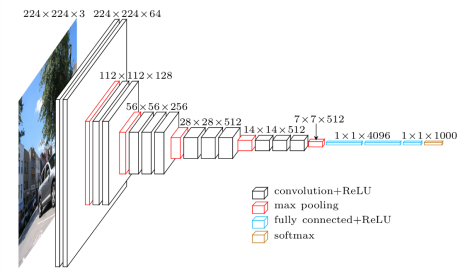
You can check here for more pretrained models https://keras.io/api/applications/. Those models could be used for different purposes such as text and image classification etc.
Here is the VGG architecture:
# training the model

model = pretrained_model((224,224,3), len(set(CLASS_NAMES)),"relu")

model.summary()

for layer in model.layers:
    print(layer, layer.trainable)

checkpointer = ModelCheckpoint(filepath='/content/drive/My Drive/COVID19/output/weights.{epoch:02d}-{val_loss:.2f}.hdf5',
                               verbose=1,
                               monitor='val_accuracy',
                               #save_weights_only=True,
                               mode='max',
                               save_freq= int(10 * STEPS_PER_EPOCH)
                               save_best_only=True)

history = model.fit(
        train_generator,
        steps_per_epoch=STEPS_PER_EPOCH,
        validation_data=validation_generator,
        validation_steps=VAL_STEPS,
        epochs=20,
        callbacks=[checkpointer])

model.save("/content/drive/My Drive/COVID19/output/google_fb_model.h5")
I hope you enjoyed this quick introduction. Let us know what you build with Keras!