MORE ON NUMPY AND IMAGE PROCESSING
Images in scikit-image are represented by NumPy ndarrays. Hence, many common operations can be achieved using standard NumPy methods for manipulating arrays. Let us get some basic ideas of numpy first.
You can click here for more details about numpy https://numpy.org/devdocs/user/quickstart.html
or https://cs231n.github.io/python-numpy-tutorial/
Disclosure: this part of tutorial relies heavily on https://numpy.org/devdocs/user/quickstart.html. You can click here for your reference.
The Basics
NumPy’s main object is the homogeneous multidimensional array. It is a table of elements (usually numbers), all of the same type, indexed by a tuple of non-negative integers. In NumPy dimensions are called axes. The number of axes is rank.
For example, the coordinates of a point in 3D space [1, 2, 1] has one axis. That axis has 3 elements in it, so we say it has a length of 3. In the example pictured below, the array has 2 axes. The first axis has a length of 2, the second axis has a length of 3.
[[ 1., 0., 0.], [ 0., 1., 2.]]
NumPy’s array class is called ndarray. It is also known by the alias array. Note that numpy.array is not the same as the Standard Python Library class array.array, which only handles one-dimensional arrays and offers less functionality. The more important attributes of an ndarray object are:
ndarray.ndim
the number of axes (dimensions) of the array.
ndarray.shape
the dimensions of the array. This is a tuple of integers indicating the size of the array in each dimension. For a matrix with n rows and m columns, shape will be (n,m). The length of the shape tuple is therefore the number of axes, ndim.
ndarray.size
the total number of elements of the array. This is equal to the product of the elements of shape.
ndarray.dtype
an object describing the type of the elements in the array. One can create or specify dtype’s using standard Python types. Additionally NumPy provides types of its own. numpy.int32, numpy.int16, and numpy.float64 are some examples.
Note1: Below is a list of all data types in NumPy and the characters used to represent them.
- i - integer
- b - boolean
- u - unsigned integer
- f - float
- c - complex float
- m - timedelta
- M - datetime
- O - object
- S - string
- U - unicode string
- V - fixed chunk of memory for other type ( void )
Note2: Information in the computer is stored as bits and bytes. A "bit" is atomic: the smallest unit of storage. A bit stores just a 0 or 1. One byte is collection of 8 bits and one byte can store one character. In general: add 1 bit, double the number of patterns. n bits yields $2^{n}$ patterns (2 to the nth power). For instance, 8 bits has 256 patterns and this is just one byte. "Byte" is the unit of information storage.
- Kilobyte, KB, about 1 thousand bytes
- Megabyte, MB, about 1 million bytes
- Gigabyte, GB, about 1 billion bytes
- Terabyte, TB, about 1 trillion bytes (rare)
check here for more info https://web.stanford.edu/class/cs101/bits-bytes.html
import numpy as np
# let us see benson's dimension
benson=np.ones((2, 2, 2))
benson
benson.ndim
benson.shape
benson.size
benson.dtype
x = np.array([1,2,3])
x
x.shape
x1=x.reshape(3,1)
x1
x1.ndim
Array Creation
There are several ways to create arrays.
For example, you can create an array from a regular Python list or tuple using the array function. The type of the resulting array is deduced from the type of the elements in the sequences.
import numpy as np
a = np.array([2,3,4])
a
a.dtype
b = np.array([1.2, 3.5, 5.1])
b.dtype
#A frequent error consists in calling array with multiple arguments, rather than providing a single sequence as an argument.
a = np.array(1,2,3,4)    # WRONG
a = np.array([1,2,3,4])  # RIGHT
# array transforms sequences of sequences into two-dimensional arrays,
# sequences of sequences of sequences into three-dimensional arrays, and so on.
a
a = np.array((1,2,3,4))
a
#The function zeros creates an array full of zeros, the function ones creates an array full of ones,
# and the function empty creates an array whose initial content is random and depends on the state of the memory.
# By default, the dtype of the created array is float64.
np.zeros((3, 4))                                # uninitialized
np.ones( (2,3,4), dtype=np.int16 ) # dtype can also be specified
np.empty( (2,3) )
# use the values you computer stores at the moement
#To create sequences of numbers, NumPy provides the arange function which is analogous to the Python built-in range, but returns an array.
np.arange( 10, 30, 5 )
from numpy import pi
np.linspace( 0, 2, 9 )                 # 9 numbers from 0 to 2
Basic Operations
Arithmetic operators on arrays apply elementwise. A new array is created and filled with the result.
a = np.array( [20,30,40,50] )
a
b = np.arange( 4 )
b
c = a-b
c
b**2
a<35
Unlike in many matrix languages, the product operator * operates elementwise in NumPy arrays. The matrix product can be performed using the @ operator (in python >=3.5) or the dot function or method:
A = np.array( [[1,1],
             [0,1]] )
B = np.array( [[2,0],
               [3,4]] )
A * B                       # elementwise product
A @ B # matrix product
A.dot(B) # another matrix product
You can also reshape numpy array like this:
b = np.arange(12)
b
b=b.reshape(3,4)
b
b.ndim
Numpy with Skimage
from skimage import data
camera = data.camera()
type(camera)
camera.shape
camera.min(), camera.max()
camera.mean()
NumPy arrays representing images can be of different integer or float numerical types. See Image data types and what they mean for more information about these types and how scikit-image treats them.https://scikit-image.org/docs/stable/user_guide/data_types.html#data-types
Image data types and what they mean In skimage, images are simply numpy arrays, which support a variety of data types 1, i.e. “dtypes”. To avoid distorting image intensities (see Rescaling intensity values), we assume that images use the following dtype ranges:
Data type Range
uint8: 0 to 255
uint16: 0 to 65535
uint32: 0 to $2^{32}$ - 1
float: -1 to 1 or 0 to 1
int8: -128 to 127
int16: -32768 to 32767
int32: -$2^{31}$ to $2^{31}$ - 1
Note that float images should be restricted to the range -1 to 1 even though the data type itself can exceed this range; all integer dtypes, on the other hand, have pixel intensities that can span the entire data type range. With a few exceptions, 64-bit (u)int images are not supported.
Functions in skimage are designed so that they accept any of these dtypes, but, for efficiency, may return an image of a different dtype (see Output types). If you need a particular dtype, skimage provides utility functions that convert dtypes and properly rescale image intensities (see Input types). You should never use astype on an image, because it violates these assumptions about the dtype range:
The following utility functions in the main package are available to developers and users:
Function name Description
img_as_float: Convert to 64-bit floating point.
img_as_ubyte: Convert to 8-bit uint.
img_as_uint: Convert to 16-bit uint.
img_as_int: Convert to 16-bit int.
These functions convert images to the desired dtype and properly rescale their values:
NumPy indexing
NumPy indexing can be used both for looking at the pixel values and to modify them:
import os
cwd=os.getcwd()
filename = os.path.join(cwd, 'benson.JPG')
from skimage import io
benson = io.imread(filename)
type(benson)
# Get the value of the pixel at the 10th row and 20th column
benson[10, 20]
Be careful! In NumPy indexing, the first dimension (camera.shape[0]) corresponds to rows, while the second (camera.shape[1]) corresponds to columns, with the origin (camera[0, 0]) at the top-left corner.
Rescale, resize, and downscale
Rescale operation resizes an image by a given scaling factor. The scaling
factor can either be a single floating point value, or multiple values - one
along each axis.
Resize serves the same purpose, but allows to specify an output image shape
instead of a scaling factor.
Downscale serves the purpose of down-sampling an n-dimensional image by
integer factors using the local mean on the elements of each block of the size
factors given as a parameter to the function.
import matplotlib.pyplot as plt
import matplotlib
matplotlib.rcParams['font.size'] = 10
from skimage import data, color
from skimage.transform import rescale, resize, downscale_local_mean

image = color.rgb2gray(benson)

image_rescaled = rescale(image, 0.25)
image_resized = resize(image, (image.shape[0] // 4, image.shape[1] // 4))

fig, axes = plt.subplots(nrows=1, ncols=3)

ax = axes.ravel()
# check here for ravel function-it returns a contiguous flattened array.
# https://numpy.org/doc/stable/reference/generated/numpy.ravel.html

ax[0].imshow(image, cmap='gray')
ax[0].set_title("Original image")

ax[1].imshow(image_rescaled, cmap='gray')
ax[1].set_title("Rescaled image")

ax[2].imshow(image_resized, cmap='gray')
ax[2].set_title("Resized image")

ax[0].set_xlim(0, 512)
ax[0].set_ylim(512, 0)
plt.tight_layout()
plt.show()

BASICS on Tensor, PyTorch, and TensorFlow
This part relies heavily on this tutorial. You can check here for more details:https://pytorch.org/tutorials/beginner/blitz/tensor_tutorial.html#sphx-glr-beginner-blitz-tensor-tutorial-py
Tensors
Tensors are similar to NumPy’s ndarrays, with the addition being that Tensors can also be used on a GPU to accelerate computing.
In order to use pytorch, you need to install first. Using pip3 install torch torchvision
import torch
# Construct a 5x3 matrix, uninitialized:
x = torch.empty(5, 3)
print(x)
An uninitialized matrix is declared, but does not contain definite known values before it is used. When an uninitialized matrix is created, whatever values were in the allocated memory at the time will appear as the initial values.
# Construct a randomly initialized matrix:
x = torch.rand(5, 3)
print(x)
# Construct a matrix filled zeros and of dtype long:
x = torch.zeros(5, 3, dtype=torch.long)
print(x)
# Construct a tensor directly from data:
x = torch.tensor([5.5, 3])
print(x)
# or create a tensor based on an existing tensor.
# These methods will reuse properties of the input tensor,
# e.g. dtype, unless new values are provided by user
x = x.new_ones(5, 3, dtype=torch.double)      # new_* methods take in sizes
print(x)

x = torch.randn_like(x, dtype=torch.float)    # override dtype!
print(x)                                      # result has the same size
# Get its size:
print(x.size())
# Converting NumPy Array to Torch Tensor
import numpy as np
a = np.ones(5)
b = torch.from_numpy(a)
np.add(a, 1, out=a)
print(a)
print(b)
# Converting a Torch Tensor to a NumPy Array
a = torch.ones(5)
print(a)
b = a.numpy()
print(b)
Let us use TensorFlow
Tensors are multi-dimensional arrays with a uniform type (called a dtype). You can see all supported dtypes at tf.dtypes.DType.
If you're familiar with NumPy, tensors are (kind of) like np.arrays.
All tensors are immutable like Python numbers and strings: you can never update the contents of a tensor, only create a new one.
You can check here for more details: https://www.tensorflow.org/guide/tensor
In order to use tensorflow, you have to install it first. https://www.tensorflow.org/install/pip
import tensorflow as tf
import numpy as np
Let's create some basic tensors.
Here is a "scalar" or "rank-0" tensor . A scalar contains a single value, and no "axes".
# This will be an int32 tensor by default; see "dtypes" below.
rank_0_tensor = tf.constant(4)
print(rank_0_tensor)
A "vector" or "rank-1" tensor is like a list of values. A vector has 1-axis:
# Let's make this a float tensor.
rank_1_tensor = tf.constant([2.0, 3.0, 4.0])
print(rank_1_tensor)
A "matrix" or "rank-2" tensor has 2-axes:
# If we want to be specific, we can set the dtype (see below) at creation time
rank_2_tensor = tf.constant([[1, 2],
                             [3, 4],
                             [5, 6]], dtype=tf.float16)
print(rank_2_tensor)
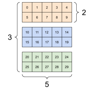
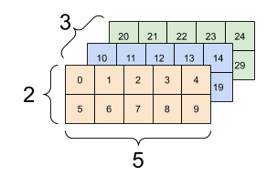
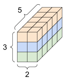
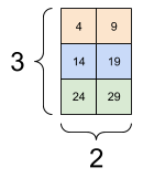
Tensors may have more axes, here is a tensor with 3-axes:
# There can be an arbitrary number of
# axes (sometimes called "dimensions")
rank_3_tensor = tf.constant([
  [[0, 1, 2, 3, 4],
   [5, 6, 7, 8, 9]],
  [[10, 11, 12, 13, 14],
   [15, 16, 17, 18, 19]],
  [[20, 21, 22, 23, 24],
   [25, 26, 27, 28, 29]],])

print(rank_3_tensor)
There are many ways you might visualize a tensor with more than 2-axes.
You can convert a tensor to a NumPy array either using np.array or the tensor.numpy method:
# use np.array
np.array(rank_2_tensor)
# use tensor.numpy
rank_2_tensor.numpy()
Some vocabulary:
- Shape: The length (number of elements) of each of the dimensions of a tensor.
- Rank: Number of tensor dimensions. A scalar has rank 0, a vector has rank 1, a matrix is rank 2.
- Axis or Dimension: A particular dimension of a tensor.
- Size: The total number of items in the tensor, the product shape vector
A rank-4 tensor, shape: [3, 2, 4, 5] |
|
|---|---|

|

|
Single-axis indexing
TensorFlow follows standard Python indexing rules, similar to indexing a list or a string in Python, and the basic rules for NumPy indexing.
- indexes start at
0 - negative indices count backwards from the end
- colons,
:, are used for slices:start:stop:step
rank_1_tensor = tf.constant([0, 1, 1, 2, 3, 5, 8, 13, 21, 34])
print(rank_1_tensor.numpy())
# Indexing with a scalar removes the dimension:
print("First:", rank_1_tensor[0].numpy())
print("Second:", rank_1_tensor[1].numpy())
print("Last:", rank_1_tensor[-1].numpy())
# Indexing with a : slice keeps the dimension:
print("Everything:", rank_1_tensor[:].numpy())
print("Before 4:", rank_1_tensor[:4].numpy())
print("From 4 to the end:", rank_1_tensor[4:].numpy())
print("From 2, before 7:", rank_1_tensor[2:7].numpy())
print("Every other item:", rank_1_tensor[::2].numpy())
print("Reversed:", rank_1_tensor[::-1].numpy())
Higher rank tensors are indexed by passing multiple indices.
The single-axis exact same rules as in the single-axis case apply to each axis independently.
# Passing an integer for each index the result is a scalar.
# Pull out a single value from a 2-rank tensor
print(rank_2_tensor)
print(rank_2_tensor[1, 1].numpy())

# tell me why it is 4 isntead of 1??
# You can index using any combination of integers and slices:
# Get row and column tensors
print("Second row:", rank_2_tensor[1, :].numpy())
print("Second column:", rank_2_tensor[:, 1].numpy())
print("Last row:", rank_2_tensor[-1, :].numpy())
print("First item in last column:", rank_2_tensor[0, -1].numpy())
print("Skip the first row:")
print(rank_2_tensor[1:, :].numpy(), "\n")
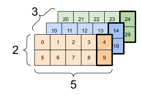
# Here is an example with a 3-axis tensor:
print(rank_3_tensor)
print(rank_3_tensor[:, :, 4])
| Selecting the last feature across all locations in each example in the batch | |
|---|---|
|
|
More on DTypes
To inspect a tf.Tensor's data type use the Tensor.dtype property.
When creating a tf.Tensor from a Python object you may optionally specify the datatype.
If you don't, TensorFlow chooses a datatype that can represent your data. TensorFlow converts Python integers to tf.int32 and Python floating point numbers to tf.float32. Otherwise TensorFlow uses the same rules NumPy uses when converting to arrays.
You can cast from type to type.
the_f64_tensor = tf.constant([2.2, 3.3, 4.4], dtype=tf.float64)
the_f16_tensor = tf.cast(the_f64_tensor, dtype=tf.float16)
# Now, cast to an uint8 and lose the decimal precision
the_u8_tensor = tf.cast(the_f16_tensor, dtype=tf.uint8)
print(the_u8_tensor)
Broadcasting
Broadcasting is a concept borrowed from the equivalent feature in NumPy. In short, under certain conditions, smaller tensors are "stretched" automatically to fit larger tensors when running combined operations on them.
The simplest and most common case is when you attempt to multiply or add a tensor to a scalar. In that case, the scalar is broadcast to be the same shape as the other argument.
x = tf.constant([1, 2, 3])

y = tf.constant(2)
z = tf.constant([2, 2, 2])
# All of these are the same computation
print(tf.multiply(x, 2))
print(x * y)
print(x * z)
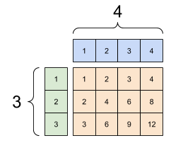
Likewise, 1-sized dimensions can be stretched out to match the other arguments. Both arguments can be stretched in the same computation.
In this case a 3x1 matrix is element-wise multiplied by a 1x4 matrix to produce a 3x4 matrix. Note how the leading 1 is optional: The shape of y is [4].
# These are the same computations
x = tf.reshape(x,[3,1])
y = tf.range(1, 5)
print(x, "\n")
print(y, "\n")
print(tf.multiply(x, y))
A broadcasted add: a [3, 1] times a [1, 4] gives a [3,4] |
|---|
|
Introduction to Variables
This part relies heavily on this tutorial: https://www.tensorflow.org/guide/variable
A TensorFlow variable is the recommended way to represent shared, persistent state your program manipulates. Variables are created and tracked via the tf.Variable class. A tf.Variable represents a tensor whose value can be changed by running ops on it. Specific ops allow you to read and modify the values of this tensor. Higher level libraries like tf.keras use tf.Variable to store model parameters.
Create a variable
To create a variable, provide an initial value. The tf.Variable will have the same dtype as the initialization value.
my_tensor = tf.constant([[1.0, 2.0], [3.0, 4.0]])
my_variable = tf.Variable(my_tensor)

# Variables can be all kinds of types, just like tensors
bool_variable = tf.Variable([False, False, False, True])
complex_variable = tf.Variable([5 + 4j, 6 + 1j])
A variable looks and acts like a tensor, and, in fact, is a data structure backed by a tf.Tensor. Like tensors, they have a dtype and a shape, and can be exported to NumPy.
print("Shape: ",my_variable.shape)
print("DType: ",my_variable.dtype)
print("As NumPy: ", my_variable.numpy())
Most tensor operations work on variables as expected, although variables cannot be reshaped.
print("A variable:",my_variable)
print("\nViewed as a tensor:", tf.convert_to_tensor(my_variable))
print("\nIndex of highest value:", tf.argmax(my_variable))

# This creates a new tensor; it does not reshape the variable.
print("\nCopying and reshaping: ", tf.reshape(my_variable, ([1,4])))
As noted above, variables are backed by tensors. You can reassign the tensor using tf.Variable.assign. Calling assign does not (usually) allocate a new tensor; instead, the existing tensor's memory is reused.
a = tf.Variable([2.0, 3.0])
# This will keep the same dtype, float32
a.assign([1, 2])
# Not allowed as it resizes the variable:
try:
  a.assign([1.0, 2.0, 3.0])
except Exception as e:
  print(f"{type(e).__name__}: {e}")
If you use a variable like a tensor in operations, you will usually operate on the backing tensor.
Creating new variables from existing variables duplicates the backing tensors. Two variables will not share the same memory.
a = tf.Variable([2.0, 3.0])
# Create b based on the value of a
b = tf.Variable(a)
a.assign([5, 6])

# a and b are different
print(a.numpy())
print(b.numpy())

# There are other versions of assign
print(a.assign_add([2,3]).numpy())  # [7. 9.]
print(a.assign_sub([7,9]).numpy())  # [0. 0.]
Let us run a demo to see why we need to understand these basic ideas.
import tensorflow as tf
import numpy as np
from tensorflow.python.training import gradient_descent


w = tf.Variable(0, dtype = tf.float32, trainable=True)

def cost():
    return w**2-10*w + 25

for _ in range(100):
    print([w.numpy(), cost().numpy()])
    gradient_descent.GradientDescentOptimizer(0.1).minimize(cost)
Now let us use TensorFlow and Keras to do a image classification Demo
Again you need to install tensorflow and keras first.
Note that you can use R or python languages..
Personaly speaking, I am shifting to R now... But I am using python and R both in this course to show you how we can benefit from these two languages in our own research.
Please click here for google tensorflow tutorial:https://www.tensorflow.org/tutorials/keras/classification
You can run it using Google Colab...
Of course you can check keras Rstudio tutorial: https://tensorflow.rstudio.com/